Review 39: Inferring Latent Dynamics Underlying Neural Population Activity via Neural Differential Equations
Inferring Latent Dynamics Underlying Neural Population Activity via Neural Differential Equations by Timothy Doyeon Kim and Carlos D. Brody
Kim, Timothy D., et al. “Inferring latent dynamics underlying neural population activity via neural differential equations.” International Conference on Machine Learning. PMLR, 2021.
- Notation : I don’t know how to use macro
\bminstead of\mathbfon this website so vector notation is going out of the window. That can be very confusing… but\mathbfis clunky. - Introduction
- Introduces generic latent model of dynamical system of neuron activity.
\(\dot{z_t} = f(z(t),u(t), t)\)
- this doesn’t not make sense to me because where is $x(t)$, or the spiking activity at time $t$ and what is the difference between $\dot{z_t}$ and $z(t)$?
- Actually, I think they mean that $\dot{z_t}$ is the subsequent measurement after reading a bit more context.
- Gives spike time formulation in terms of Poisson process as in previous post (LFADS).
- Drawbacks to LFADS
- RNN is high dimensional making it mostly black box until you get factors.
- requires many trials to train.
- the initial state of the RNN and the external input stimuli completely determine the state trajectory.
- In reality, the same stimuli may not give rise to the same output … the brain is not deterministic.
- Also different exogenous stimuli can give rise to the same output… not sure if these matter as much here.
- This paper introduces a low dimensional model that uses neural ODES (Chen et al. 2018) to model population dynamics.
- This means we can find the fixed points using the jacobian of the diff. eqs. of this model like Sussillo 2013 (see review 36).
- Outperforms LFADS in single trial tasks.
- Latent trajectories are sampled then computed using ODE Solver so they are not deterministic.
- Model gives phase portraits that can reconstruct flow field (is it flow field or curl field or vector field… IDK terminology here).
- Introduces generic latent model of dynamical system of neuron activity.
\(\dot{z_t} = f(z(t),u(t), t)\)
- Background
- Poisson Linear Dynamical System (PLDS)
\(\begin{aligned}
&z_0 = \mathcal{N}(\mu_{z_0}, Q_0 ) \hspace{20pt} \tiny{\textit{sample initial latent state}} \\
\eta_t \sim \mathcal{N}(0,Q_t) \tiny{\textit{sample noise?}} \\
&z_t = Az_{t-1} + Bu_t + \eta_t \tiny{\textit{linear model for next latent state}} \\
&\lambda_t = exp(C_k z_t + \eta_t) \tiny{\textit{find poisson rate}} \\
&x_{t,n} = \text{poisson}(\delta t\lambda_{t,n}) \tiny{\textit{sample spike trains}}
\end{aligned}\)
- though they use $k$ to denote instantaneous measurements instead of $t$.
- This is solved via EM… is guess on the latent distributions $Q_0$ and $Q_t$ and then on the linear regression weights $A$,$B$, and $C_k$.
- 2.2 LFADS - latent factor analysis via dynamical systems. I’ll skip this background since it is covered thoroughly in review 38, (TODO: add links) the previous review.
- Neural ODE
- Instead of using feed-forward net to solve latent trajectory, one can use ordinary differential equations.
- Instead of an explicit ODE solve method, (Chen 2018) proposes using adjoint states to approximate the gradient of the loss of the ODES (latent ODEs that is).
- Adjoint state for latent traj: $a(t) = \frac{d\mathcal{L}}{dz(t)}$
- Respective ODE $\frac{da(t)}{dt}= -a(t) \frac{\partial f_{\psi}(z(t),t)}{\partial z(t)}$
- Adjoint state for approx. of loss $a_{\psi}(t) = \frac{d\mathcal{L}}{d{\psi}}$
- Respective ODE $\frac{da_\psi(t)}{dt}= -a(t) \frac{\partial f_{\psi}(z(t),t)}{\partial \psi}$
- 2.5. Pulsatile Evidence Accumulation in Perceptual Decision-Making
- Rodent has clicks on the left and right side and is rewarded for choosing what side had the most clicks.
- Model by
\(dz = \lambda z dt + \delta_R(C^R + \eta_R)dt + \delta_l(C^L + \eta_L)dt + \sigma_z dW\)
- where $\eta_L$ and $\eta_R$ $\sim \mathcal{N}(0,\sigma)$
- and $C^L$ and $C^R$ represent update frequencies.
- Do not understand $dW$ (how would there be deriv. w.r.t to W if there’s no W in the eq.??)
- Poisson Linear Dynamical System (PLDS)
\(\begin{aligned}
&z_0 = \mathcal{N}(\mu_{z_0}, Q_0 ) \hspace{20pt} \tiny{\textit{sample initial latent state}} \\
\eta_t \sim \mathcal{N}(0,Q_t) \tiny{\textit{sample noise?}} \\
&z_t = Az_{t-1} + Bu_t + \eta_t \tiny{\textit{linear model for next latent state}} \\
&\lambda_t = exp(C_k z_t + \eta_t) \tiny{\textit{find poisson rate}} \\
&x_{t,n} = \text{poisson}(\delta t\lambda_{t,n}) \tiny{\textit{sample spike trains}}
\end{aligned}\)
- PLNDS
- log-likelihood function ($p_{\Theta}(t_x \mid u)$) is the likelihood of spike times for N observed neurons and $u$ is the input.
- parameters of the model are $\Theta = [\theta,\phi]$ where $\theta$ are ODE solver params and $\phi$ are variational params.
- Then log-lik = \(\begin{equation} \mathcal{L} = \mathbb{E}_{q}[p_{\theta}(t_x \mid u, z)] + KL(p_{\theta}(z \mid u, t_x) || q_{\phi}(z \mid t_x, u)) \end{equation}\)
- And likelihood is reduced to
\(\begin{equation}
\mathbb{E}_{q}[p_{\theta}(t_x \mid u, z)] = \mathbb{E}_{q}[p_{\theta}(t_x \mid \lambda)] = \sum_{n=1}^{N} \mathbb{E}_{q}[log(p_{\theta}(t_x^{(n)}))] \mid \lambda_n)] \\
\text{ where }
\mathbb{E}_{q}[log(p_{\theta}(t_x^{(n)}))] = - \int_{\tau} \lambda_n t dt + \sum_{i=1}^{\alpha(n)} log \lambda_n t_{x,i}^{(n)}
\end{equation}\)
- not quite sure how we get the final expansion of log likelihood for $p(\t_x \mid \lambda_t)$. I thought it would be like a binary crossentropy kinda thing but the integral over $\lambda_n$ is throwing me off.
- Going to skip the part about computing adjoints and computing the KL Div. for adjoints… I imagine this derivation is from Chen 2018.
-
Experiments
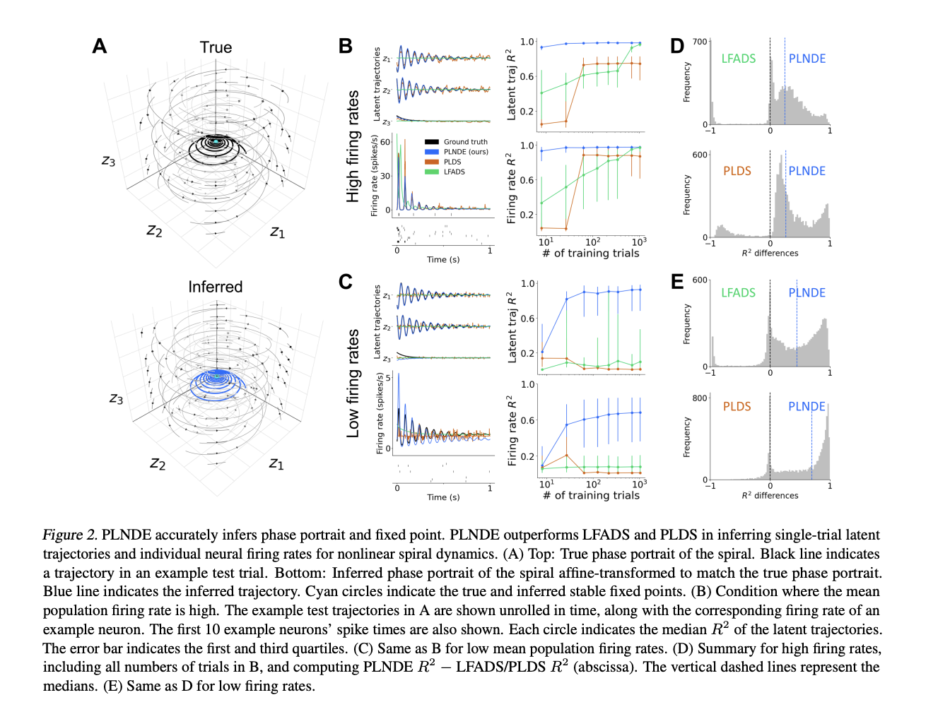
- PLNDS accurately reconstructs phase portrait spiral resulting from linear dynamical system of eq. similar to that of Brunton 2016.
- Fixed points found using Newtons method and autodiff of FNN (fig 2A).
- PLNDE outperformed LFADS and PLDS in firing rate reconstruction accuracy experiments where number of training trials and firing rates varied (fig 2B / 2C). This is demonstrated in $R^2$ on the right panel and reconstruction of latent trajectories on the left panel for 2B and 2C. The trend here shows a very high correlation for PLNDE with actual firing rate in the early trials for high activity. This drops off for low activity but eventually recovers after many trials. This is not the case for PLDS and LFADS.
- Paper provides a method for finding the right number of latent dimensions using validation loss.
- “We found that PLNDE can accurately infer the phase portrait of FitzHugh-Nagumo, capturing the limit cycle and the unstable fixed point. [and] 4.2), PLNDE can infer the phase portrait of the mutual inhibition dynamics, correctly identifying the two stable and one unstable fixed “
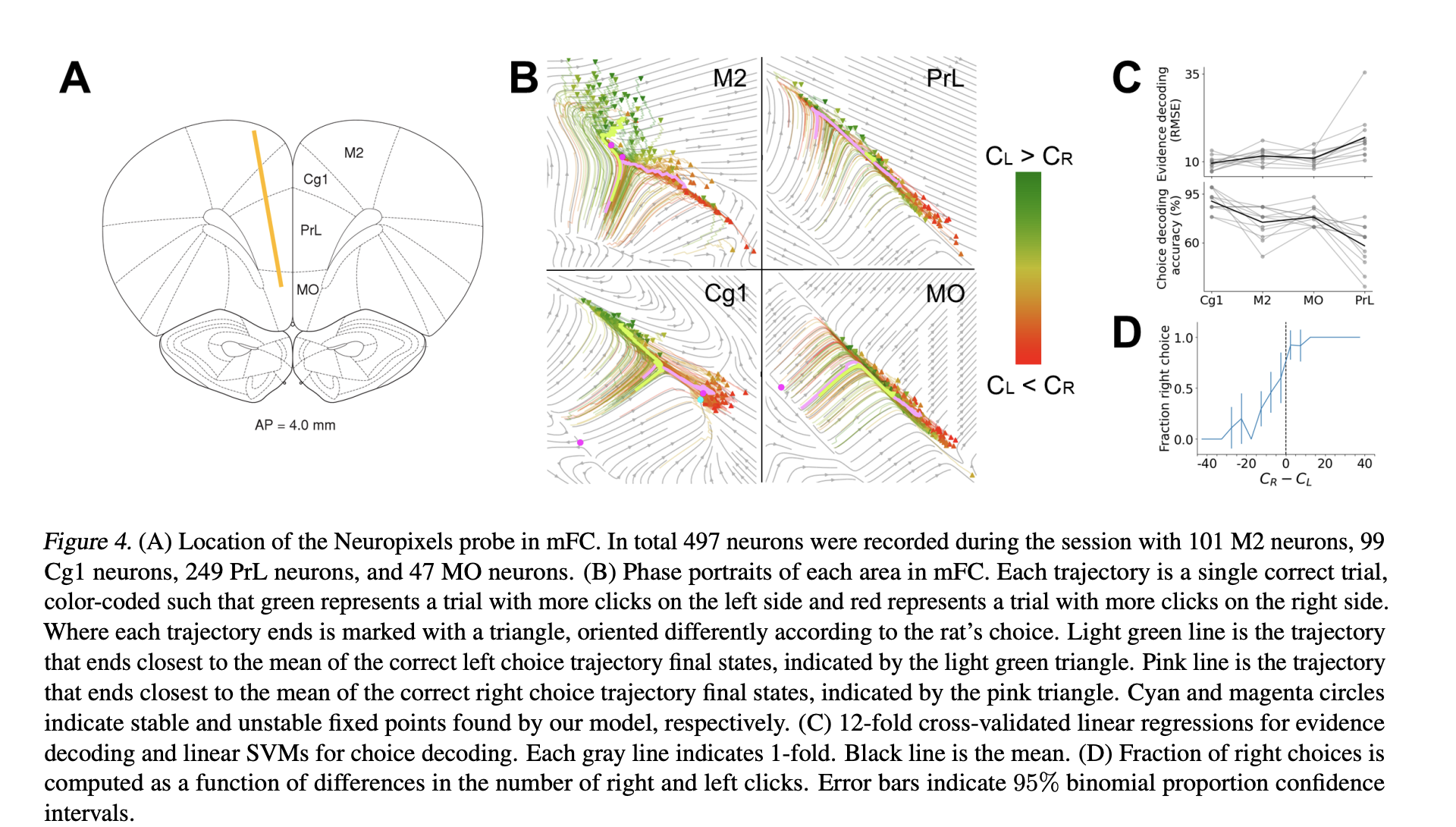
- Next they fit PLNDE to various regions (prelimibic, secondary motor, pre-frontal) of a rat in a decision making task.
- PLNDE confirms importance of decision making regions while also creating latent space phase portrait. That would be figure B below.
- Discussion
- PLNDE does not provide a measure of confidence in it’s estimate of the phase portrait. Thus a measure of caution should be used in the underlying assumptions about the stationarity of the system and the portrait being used to describe the system.
- Model has less parameters than LFADS.
- We may also consider amortizing posterior inference of our model by having, for example, an RNN encoder like (6), ODE-RNN encoder (Rubanova et al., 2019).
- Final point about hyperparm optimization.