Review 38: Latent Factor Analysis via Dynamical Systems (LFADS)

LFADS - Latent Factor Analysis via Dynamical Systems by David Sussillo and Chethan Pandarinath

Sussillo, David, et al. “Lfads-latent factor analysis via dynamical systems.” arXiv preprint arXiv:1608.06315 (2016).

Notation : I don’t know how to use macro \bm instead of \mathbf on this website so vector notation is going out of the window. That can be very confusing… but \mathbf is clunky.
Introduction
- peri-stimulus time histogram (PTSH) as the common approach to analyzing high dimensional spike train data.
- LFADS, or latent factor analysis via dynamical systems, takes a sequenetial perspective, as opposed to input -> feedforward -> output), but also models external inputs.
- Goal of inferring smooth dynamics of single trial from neural population data.
- Also provides:
  - a set of low-rank latent factors
  - initial conditions
  - and infers inputs.
- “LFADS is designed to infer such inputs on the basis of the recorded data alone.”
LFADS Model
- Uses a variational autoencoder (VAE) to model data $x$ and it’s relationship latent variables $z$ using prior $p(z)$ and conditional $p(x \mid z)$ . Naturally need to train approximation $q(z \mid x)$ of true posterior $p(z \mid x)$ using $\frac{p(x \mid z)p(z)}{p(x)}$.
- $\hat{z}$ is a sample from $q$ which can be seen as an encoded version of data $x$ and the true posterior $p(x \mid x)$ can be seen as the decoder.
  - See previous review for more details on VAE and KL divergence as a method for normalization.
- Notation:
  - $v = W(u)$ is an affine transformation from $u$ to $v$.
  - RNN update is $state_t = RNN(state_{t-1}, input_t)$.
  - Data is $x_{1:t}$ spike trains from D neurons and auxilliary set of observed variables $a_{1:t}$.
  - Assuming $x_{1:t}$ are sampled from Poisson process with rates $r_{1:t}$. Latent factors are $f_{1:t}$.
  - Inferred input to network $u_{1:t}$
    - $ z = {g_0,u_{1:t}}$
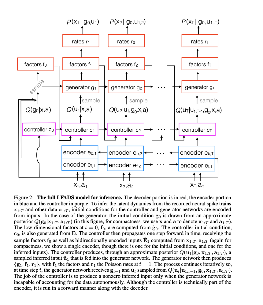
- LFADS generator / decoder
  - rates are determined as $r_{1:t} = W^{\text{rate}}(exp(f_{1:t}))$.
  - start by sampling intitial state $\tilde{g_0}$ from prior $p(g_0)$ then:
  \[\begin{aligned} \hat{u} \sim P(u) \hspace{20pt} \tiny{\textit{sample input}} \\ &g_t = RNN^{gen}(g_{t-1}, \hat{u}) \hspace{20pt} \tiny{\textit{generate next hidden state}} \\ &f_t = W^{fac}g_t \hspace{20pt} \tiny{\textit{affine transform to factors}} \\ &r_t = exp(W^{rate}(f_t)) \hspace{20pt} \tiny{\textit{infer rate from factors}} \\ &x_t \sim Poisson(x_t \mid r_t) \hspace{20pt} \tiny{\textit{sample spike outpts / decode}} \end{aligned}\]
- LFADS encoder
  - both $g_0$ and $u_t$ are diagonal gaussians with mean and var.
  - $Q(g_{0} \mid x, a)$ with mean and var in terms of $E$: $\begin{aligned} &\mu^{g_0} = W^{\mu_{g_0}}(E) &\sigma^{g_0} = exp(\frac{1}{2}W^{\sigma^{g_0}}(E)) \end{aligned}$
    - So far this is my weakest point of understanding: it seems like E is a forwards/backwards trajectory and that distribution Q is defined by an affine transformation to that state.
      - This is where I think Neural ODE and Latent ODE have application since the affine transformation is not a principled way to from positions $E$ to distribution $q$.
      - Same thing with the controller.
    - E $[e_1^{b}, e_{T}^{f}]$ is obtained through forward $e_{t}^{b}$ and backward $e_{t}^{f}$ RNN passes.
  - Then $u_t$ is defined in a similar way, (but also include a RNN controller?), and different trainable parameters. Thus giving $\tilde{E}_t$. Notice that it is no longer a pair of ending states of backward/forwards pass but a continuous trajectory over time $t$.
    - Previously we generated $g_0$ as an initial condition.
  - $\tilde{E}_t$ and latent factor $f_t$ then pass through controller : $c_t = RNN^{conn}(c_{t-1}, [\tilde{E}_t, f_{t-1}])$.
  - Finally inferred input $\hat{u}_t$ is drawn from a distribution parameterized by an affine transformation of the controller network state $c_t$ defined in the bullet above. $\begin{aligned} &\hat{u}_t \sim Q(u_t \mid \mu_t^u, \sigma_t^u) \\ &\mu_t^u = W^{\mu^u} c_t \\ &\sigma_t^u = exp(\frac{1}{2} W^{\sigma^u} c_t) \end{aligned}$
- Ok now lets put the whole thing together in one set of eq. $\begin{align} &c_t = RNN^{conn}(c_{t-1}, [ \tilde{E}_t,f_{t-1} ]) \hspace{20pt} \tiny{\textit{get controller state from RNN}} \\ &\mu_t^u = W^{\mu^u} c_t \hspace{20pt} \tiny{\textit{affine transformation to controller state for } \mu_t^u}\\ &\sigma_t^u = exp(\frac{1}{2} W^{\sigma^u} c_t) \hspace{20pt} \tiny{\textit{affine transformation to controller state for } \sigma_t^u} \\ &\hat{u}_t \sim Q(u_t \mid \mu_t^u, \sigma_t^u) \hspace{20pt} \tiny{\textit{sample input}} \\ &g_t = RNN^{gen}(g_{t-1}, \hat{u}) \hspace{20pt} \tiny{\textit{generate next hidden state}} \\ &f_t = W^{fac}g_t \hspace{20pt} \tiny{\textit{affine transform to factors}} \\ &r_t = exp(W^{rate}(f_t)) \hspace{20pt} \tiny{\textit{infer rate from factors}} \\ &x_t \sim Poisson(x_t \mid r_t) \hspace{20pt} \tiny{\textit{sample spike outpts / decode}} \end{align}$
- technically this isn’t the whole thing, just the generative process since encoder isn’t parameterized here.
- just figured out how to left align these equations on this website and it’s so satisfying. Previously they were center aligned.
Loss function
- $ log P(x_{1:T}) \geq \mathcal{L} = \mathcal{L}^x - \mathcal{L}^{kl} $
- $\mathcal{L}^{kl} $ is two KL divergence terms.
  - one on the approximated posterior distribution of the inputs $u_t$ .
  - and one on the starting point state $g_0$ .
- $\mathcal{L}^x = \sum_{t=1}^{T} log(\text{Poisson}(x_t \mid r_t)$.
Previous work
- Kalman filters, VRAE (recurrent VAE).
- Generalized Linear Model with Poisson Process.
- Gaussian Process Factor Analysis.
Results
- Experiments include:
  - Lorenz system
    - LFADS latents do the best in reconstruction of 3 dimensional state space $y_1,y_2, y_3$
  - Inferring dynamics of chaotic RNN
  - Inferring inputs of chaotic RNN
    - Trials with $\gamma$ controlling how chaotic activity is.
Next directions

Sussilo 2016

There are some obvious extensions and future directions to explore. First, an emissions model relevant to calcium imaging would be extremely useful for inferring neural firing rate dynamics underlying calcium signals. Second, in this contribution we implemented LFADS as a “smoother”, in Kalman filter language, that cannot run in real time. It would be interesting to adapt LFADS as a “filter” that could. Third, the LFADS generator could clearly be strengthed by stacking recurrent layers or adding a feed-forward deep net before the emissions distribution at each time step. Another extension would be to learn the dimensions of the inferred input and temporal factors automatically, instead of having them specified as predetermined hyper-parameters (e.g. nuclear norm minimization on the respective matrices). Finally, we can imagine an LFADS-type algorithm that leans more towards the feed-forward side of computation, but still has some recurrence. An application would be, for example, to explain short-term effects in visual processing. In this setting, the information transfer along the temporal dimension could be limited while expanding the information flow in the feed-forward direction.