Review 37: Auto-Encoding Variational Bayes
Auto-Encoding Variational Bayes by Diederik P. Kingma and Max Welling
Kingma, Diederik P., and Max Welling. “Auto-encoding variational bayes.” arXiv preprint arXiv:1312.6114 (2013).
- Notation : I don’t know how to use macro
\bminstead of\mathbfon this website so vector notation is going out of the window. That can be very confusing… but\mathbfis clunky. - Introduction
- They show how a simple reparamterization of the variational lower bound yields a simple differntiable unbiased estimator of the lower bound in SGVB (stochastic gradient variational bayes).
- The approximate posterior inference model can be used for representation, denoising, recgoniztion, visualization etc. and they call it Variational auto-encoder.
- Methods
-
- Problem setting
- Consider dataset $ X = { [x^{(i)}] }^N_{i=1} $ consisting of N iid samples of some contininous or discrete variable $x$.
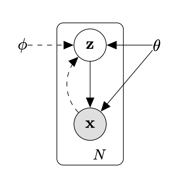
- Data is generated by some by some process represented by latent variable $z$ with prior $z \sim p_{\theta^*}(z)$ and likelihood $x \sim p_{\theta^*}(x \mid z)$. Where distribution $\theta^*$ and latent R.V. $z$ are unknown.
- Paper does not make several assumptions resulting in a setting characterized by:
- Intractability: Assume we cannot explictly compute the integral of the marginal likelihood $p_{\theta}(x)= \int p_{\theta}(x \mid z) p_{\theta}(z) dz$.
- Dataset is too large to sample solutions to MAP using Monte Carlo EM.
- So they propose a solution to 3 real world problems in this setting.
- Efficient maximum likelihood (ML) of maximum a posteriori (MAP) of parameters of $\theta$
- Inference on latent variable $z$ given $x$ and estimated parameters of $\theta$.
- Efficient approximate marginal inference of the variable $x$.
- Introduce a “recognition model” or appromximation of the true posterior $p_{\theta}(z \mid x)$ as $q_{\theta}(z \mid x)$.
- Variational Bound
- The likelihood of a given sample is \(log p_{\theta}(x^{(i)}) = KL(q_{\theta}(z \mid x^{(i}) || p_{\theta}(z \mid x^{(i)}) + \mathcal{L}(\theta, \phi ; x^{(i)})\) for $ i = 1 … N$ datapoints.
- Then we can replace $ \mathcal{L}(\theta, \phi ; x^{(i)}) $ with \(\mathbb{E}_{ q^{\phi}(z \mid x) } [- log q_{ \theta }(z \mid x) + log p_{\theta}(z, x)]\)
- How does this derivation work for the variational lower bound?
- Then the final equation we get for the variatonal lower bound is: \begin{equation} log p_{\theta}(x^{(i)}) = KL(q_{\theta}(z \mid x^{(i}) || p_{\theta}(z \mid x^{(i)}) + \ \mathbb{E}_{q^{\phi}(z \mid x)} [- log q_{ \theta }(z \mid x) + log p_{\theta}(z, x)]] \end{equation}
- Gradient w.r.t. to $\phi$ the recognition model parameters is tricky to compute because you’d have to use naive monte carlo gradient estimator.
- The SGVB estimator and the AEVB algorithm
- This is the good part now. They reparameterize $\tilde{z} = q_{\phi}(z \mid x)$ using a differentiable equation $ g_{\phi}(\epsilon, x)$ ! where $\epsilon$ is a random noise variable. So: \(\tilde{z} = g_{\phi}(\epsilon, x) \ \text{with} \ \epsilon \sim P(\epsilon)\)
- Then we can replace $q_{phi}(z \mid x)$ in equation 1 with function $g_{\phi}(\epsilon, x)$. Except now the monte carlo estimate of expectation is conditioned on $p(\epsilon)$ now, because that is the underlying distribution.
- Now we using stochastic variational estimate: $\tilde{\mathcal{L}}^A(\theta, \phi ; x^{(i)}) $
- Thus we finally get to the form of the Stochastic Gradient Variational Bayes (SGVB) estimator: \begin{equation} \tilde{\mathcal{L}}^A(\theta, \phi ; x^{(i)}) = \frac{1}{L} \sum_{l=1}^L log_{p_{\theta}} (x^{(i)}, z^{(i,l)}) - log_{p_{\theta}}(z^{(i,l)} \mid x^{(i)}) \end{equation} where $z^{(i,l)} = g(\epsilon^{i,l},x^{(i)}) $ and $\epsilon^{l} \sim p(\epsilon)$ .
- Then there is the regularized version of SGVB which uses KL divergence to ground the variational distribution $q_{\theta}$ with a prior distribution. This has the form: \begin{equation} \tilde{\mathcal{L}}^A(\theta, \phi ; x^{(i)}) = KL(q_{\theta}(z \mid x^{(i}) || p_{\theta}(z \mid x^{(i)}) + \ \frac{1}{L} \sum_{l=1}^L log_{p_{\theta}} (x^{(i)}, z^{(i,l)}) - log_{p_{\theta}}(z^{(i,l)} \mid x^{(i)}) \end{equation}.
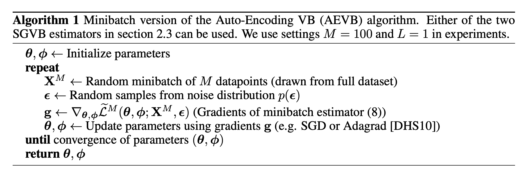
- The next part of this paper describes how to do minibatch updates using an optimizer like SGD / ADAM because we can now take gradients w.r.t to $\theta$ and $\phi$.
- In equation 3 the first term serves as a regularizer and the second term serves as a reconstruction loss as it produces a generative model of datapoint $x^{(i)}$ given $z^{(i,l)}$ .
- The reparameterization trick
- If $z$ is a continuous r.v. sampled from $q_{\phi}$(z \mid x)$, then they express $z$ in terms of a deterministic variable $z = g(\epsilon, x)$ with an indpendent marginal $p(\phi)$.
- Then they provide a proof for why monte carlo estimate of expectation is differentiable w.r.t. $\phi$.
- But still, the trick is hard to understand intuitively since changing the parameters of $q_{\phi}$ doesn’t change the indpendent marginal $p(\epsilon)$ which is some noise.
- On that note, the rest of this section goes on to describe the reasonable choices for $p(\epsilon)$.
- Variatonal AutoEncoder
- Start by assuming variational approximate posterior is multivariate gaussian s.t.: $ log q_{\phi}( z \mid x^{(i)}) = \mathcal{N}(z; \mu^{(i)}, \sigma^{2(i)} I)$ where the mean and s.d. of the approximate posterior, $\mu^{(i)}$ and $\sigma^{i}$ are outputs of the encoding MLP, i.e. nonlinear functions of datapoint $x^{(i)}$ and variatonal parameters $\phi$.
- Then the resulting estimator is: \begin{equation} \mathcal{L}(\theta, \phi ; x^{(i)}) \simeq \frac{1}{2} \sum_{j=1}{J} ((log(\sigma_{j}^{(i)})^ 2) + (\mu_{j}^{(i)})^ 2) - (\sigma_{j}^{(i)})^ 2)) + \frac{1}{L} \sum_{l=1}^L p_{\theta}(x^{(i)} \mid z^{(i,l)}) \end{equation}
- The relational works section is pretty interesting because it shows just how novel this method is. There does seem to have been some work, called wake-sleep, on recognition for latent variable model for an approximation of the true posterior, but certainly it did not involve gradient descent. Besides that, related work is auto-encoders.
- Experiments.
- MNIST
- outperforms wake-sleep benchmark even with only 3 latent variables.
- lower likelihood than Frey face.
- Frey Face
- outperforms wake-sleep benchmark even with only 3 latent variables.
- much higher likelihood model
- Adding more latent variables never actually decreases evidence lower bound which is kinda crazy given they usee 200 latent variables.
- Something that would be abosolutely impossible if using MCMC approximation.
- Figure 3 shows an excellent result w.r.t. to scale. That is simply: using less latent variables they can use MCMC to approximate posterior but the effectiveness does not scale nearly as well with more training data. Showing scalability of the AEVB method is an excellent idea.

- MNIST
- Future work
Kingma and Welling 2013
there are plenty of future directions: (i) learning hierarchical generative architectures with deep neural networks (e.g. convolutional networks) used for the encoders and decoders, trained jointly with AEVB; (ii) time-series models (i.e. dynamic Bayesian networks); (iii) application of SGVB to the global parameters; (iv) supervised models with latent variables, useful for learning complicated noise distributions.
- We like (ii)!
-