Review 36: Opening the Black Box: Low-Dimensional Dynamics in High-Dimensional Recurrent Neural Networks

Opening the Black Box: Low-Dimensional Dynamics in High-Dimensional Recurrent Neural Networks by David Sussillo and Omri Barak

Sussillo, David, and Omri Barak. “Opening the black box: low-dimensional dynamics in high-dimensional recurrent neural networks.” Neural computation 25.3 (2013): 626-649.

Notation : I don’t know how to use macro \bm instead of \mathbf on this website so vector notation is going out of the window. That can be very confusing… but \mathbf is clunky.
Introduction
- View of RNN as a non-linear dynamical system (NLDS).
- Phase space: Just a more specifc term than state space, instead of general description of all possible states, phase space defines a state as a set of coordinates.
- Fixed points: Coordinates in the phase space that exhibit zero motion. extends to Slow points.
  - Stable or unstable (or attractor v. repeller), meaning system converges towards or away from these points.
  - mode: independent pattern of activity that arises around fixed point when the linear system is diagonalized.
- Hypothesis is that RNN == NLDS, but at slow points, linearization is valid. Paper provides principled approach to finding regions with slow points, then linearizes arround each slow point, and then relates interaction between regions.
- Technique introduced allows id. of attractors, repellers, and saddle ponts.
Linear approximations
- a system of diff. eqs.: $ \dot{x} = F(x) $ and trying to find points, $ x^{*} $ such that $ | F(x^{*}) \partial x | \geq F(x^{*}) $ and $ | F(x^{*}) \partial x | \geq | \frac{1}{2} \partial x F’‘(x^{*}) \partial x | $.
- The way I understand this is that perturbations induce a linear rate of change in the value of the system and the rate of change in the system.
- Speed, or kinetic energy, of the system is : $ q(x) = \frac{1}{2}|F(x)|^2 $, which is useful because it is a scalar that can be optimized, q = 0 only at fixed points, and gradient and hessian of q are amenable to finding minimum values that are not fixed points (so they are saddle points?).
  - don’t fully understand how the conditions for minimum are derived but moving on for now.
- 2 - d example:
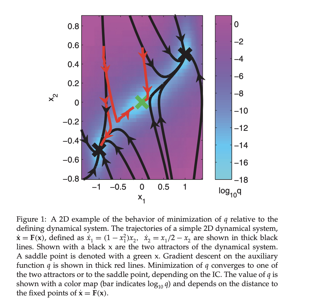
  - defined as dynamical system: \begin{equation} \dot{x_1} = (1 - x_1^2)x_2 \end{equation} \begin{equation} \dot{x_2} = x_1 / 2 - x_2 \end{equation}
  - The system has three fixed points: a saddle at (0, 0) and two attractors at (1, 1/2) and (−1, −1/2).
  - Here is the figure used to describe this dynamical system. I find it useful because it shows how differnt ICs (inital conditions) can converge to different fixed points and does a decent job of showing the difference between saddle and fixed point.
- RNN formulation
  - $\mathbf{x}$ is the vector of activations and $\r(x_i)$ is the firing rate for neuron $i$ \begin{equation} \dot{x_i} = -x_i \sum_{k}^N j_{ik}r_k + \sum_{k}{N} B_{ik}u_k r_i = h(x_i) \end{equation}
  - The recurrence of the network is defined by the matrix J, and the network receives the I-dimensional input u through the synaptic weight matrix B.
- 3 bit flip flop
  - TODO I do not understand many things about the 3 bit task. So I just write open questions here instead.
    - Do the 3 units have a sequential relationship?
    - The input pulses are real valued? How are they thresholded?
    - In figure 2, are the inputs colored or the outputs? Seem like the outputs are colored, but it’s still hard to relate them.
  - Still, I need to give best description of the system so we’ll go ahead.
  - $2^3 = 8$ possible memories. Random impulses hit each bit and either confirm the sign (because it matched +1,-1) or flip sign from +1 to -1.
  - modeled with echostate RNN trained using FORCE (Sussillo & Abbot 2007) and trained using random init. weights and 600 different starting points (ICs). Fixed point finder resulted in 26 distinct fixed points and then they analyze these w/ linear stabiility anaylsis described above.
  - important there are 8 attractors for every memory state.
  - Sussillo and Barak 2013
    
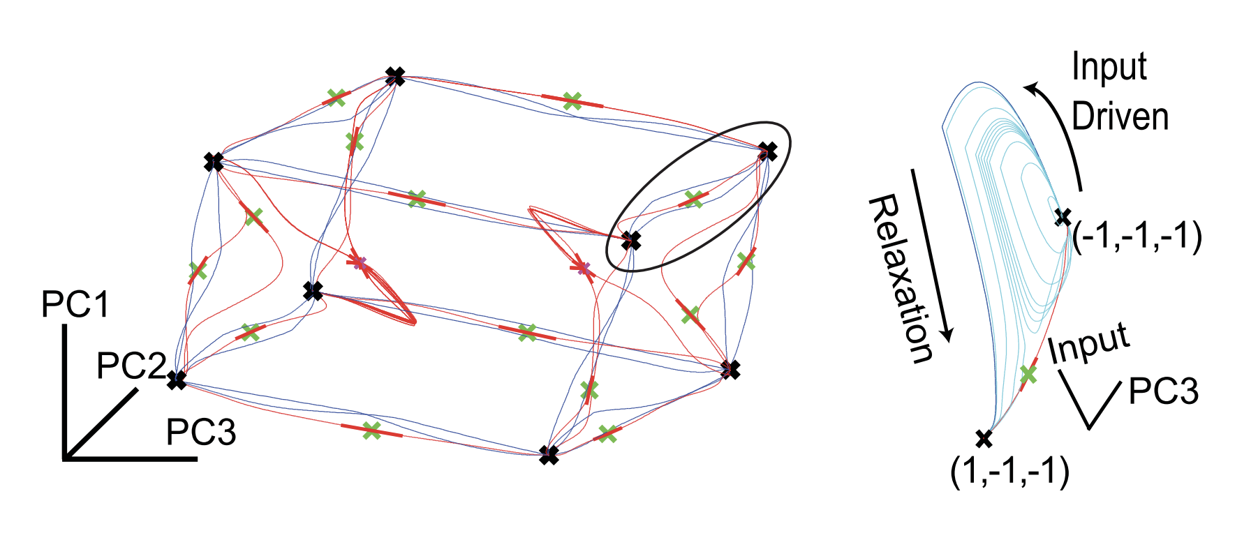
    Figure 3: Low-dimensional phase space representation of 3-bit flip-flop task. (Left) The eight memory states are shown as black x. In blue are shown all 24 1-bit transitions between the eight memory states of the 3-bit flip-flop. The saddle fixed points with one unstable dimension are shown with green x. A thick red line denotes the dimension of instability of these saddle points. In thin red are the network trajectories started just off the unstable dimensions of the saddle points. These are heteroclinic orbits between the saddles that decide the boundaries and the attractor fixed points that represent the memories. Finally, the pink x show other fixed points, all with four unstable dimensions. Thick red lines show these dimensions of instability, and thin red lines show network trajectories started just off the fixed points in these unstable dimensions. (Right) Demonstration that a saddle point mediates the transitions between attractors. The input for a transition (circled region in left panel) was varied from 0 to 1, and the network dynamics are shown (blue for normal input pulse and cyan for the rest). As the input pulse increased in value, the network came ever closer to the saddle and then finally transitioned to the new attractor state.
  - System uses saddle points to mediate transition from one memory to another.
  - Though most transition from memory states are fairly straightforward, there are some unstable trajectories that appear to serve no purpose (pink fixed points).
  - Without explicit design of a network for a particular phase space, there can be redundant or multiple fixed points between two attractor states.
- Sine wave generator
  - Network that produces a target sine wave for a given frequency from 1-51 frequency values.
  - linearized system had only two unstable dimensions.
  - Is it a surprising result that there is a fixed point corresponding to the 51 freq. values? Obviously we know some of them still result in regions of interest, but is the 1-1 correspondence implied by the task or not?
    - These regions are rigorously verified by norm of linear term agreeing with conditions (idk the eq. # above, but it’s the ones under “linear approximations” section).
    - So I guess that is not necessarily implied by the fixed point analysis.
- Beyond fixed points
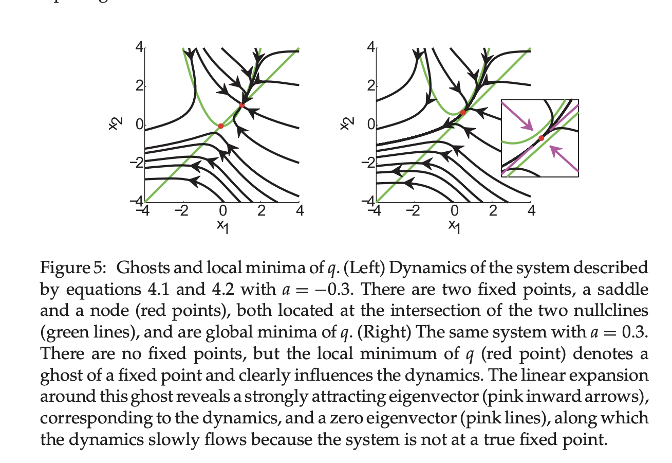
  - saddle points found by $q$ (“linear approximations” section) also provide insight system because linear term is dominating even if zero order of taylor expansion != 0. They term these points ghost points (or slow points) and state that even if they are not mediating transitions directly like fixed points, they are influencing the tracjectory of the system as shown below.
    - I thought zero-order term was linear? And first or second order might not = 0.
  - paper includes some examples and formalizaiton of linear dynamics around this point.
- Approximate plane attractor
  - This example further demonstrates the utility of finding saddle points using $q$. Because this is a summary I won’t explain the approximate plane attractor in too much detail.
  - The gist is that it is a 2 point moving average task which means two values need to be stored in memory.
  - 100dim. RNN slow points ($q \leq 1e-4$) actually created a two dimensional manifold.
  - “Ablation study” so to speak done by replacing slow points with linear time-varying dynamical system (LTVDS) with very low mean squared error on transition states.
  - finally, they show the method is robust to perturbations in RNN and doesn’t rely on a finely tuned RNN.
    - This is important to show (something a reviewer might have asked for), but I will not cover it here.
- Discussion
  - Open points for future work include
    - generalization to higher dimensional inputs and tasks.
    - May provide insight into observed experimental findings of low-dim. dynamics of experimental neuroscience.
      - This is the one I am interested in!
    - Applying this technique to spiking models.
      - Also this…